Deep Learning Model

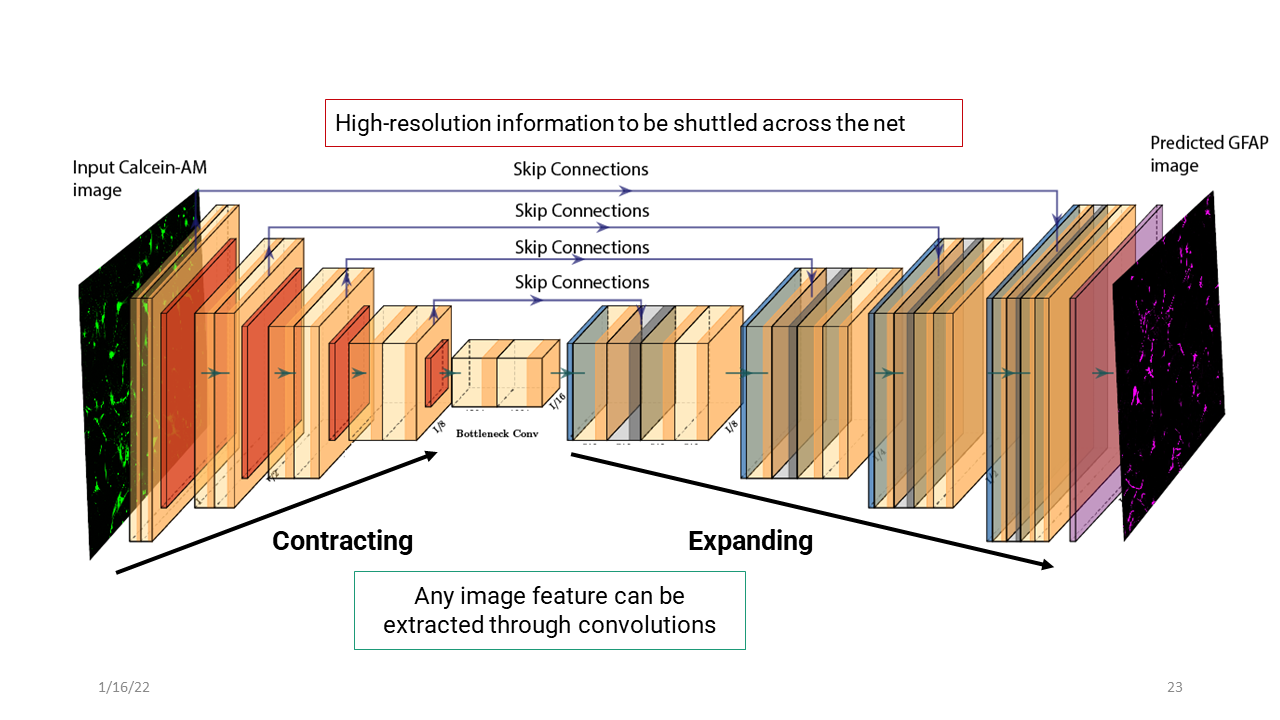
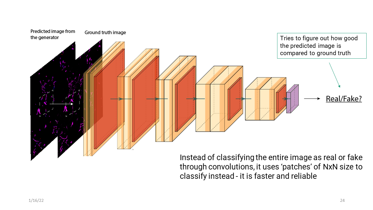
Here is the overall deep learning model architecture that I will be using to . It actually comprises of two Convolutional neural networks, where one works as a generator and the other, a discriminator. The generator outputs predicted image given an input. The dsicriminator then takes this in and the ground truth image, and tries to see if it is good enough, or what they classify as real or fake. This information is relayed to the generator so that it can make better predictions.

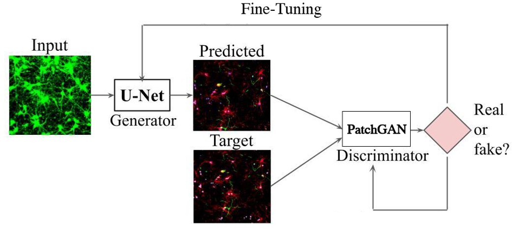
I want to give you a closer look into each CNN and give you a brief overview as to how it works. The generator is a U-net based CNN, and what it does is it essentially boils down the input image, contracting it as much as it can using bunch of filters and convolutions to get the essence of the image and store it to a feature vector. This vector would have information about the edges, gradients, shapes etc. And then it takes this feature vector, and tries to expand it by using transpose convolutions. The skip connections shown below are the hallmark of U-Net based networks. What it does is, whatever information we have at these levels, it gets shuttled across the net and is used in the expansion process. This allows feature maps at these levels to be integrated, which ensures that the finer details are preserved in the predicted image.

Discriminator network is based on a PatchGAN classifier and it basically tries to determine the similarity between the two images locally at the scale of ‘patches’. It goes through a similar convolutional process and essentially gives you whether the predicted image is as good as the ground truth and whether it was able to fool the network. So this wraps up the deep learning portion of my thesis.

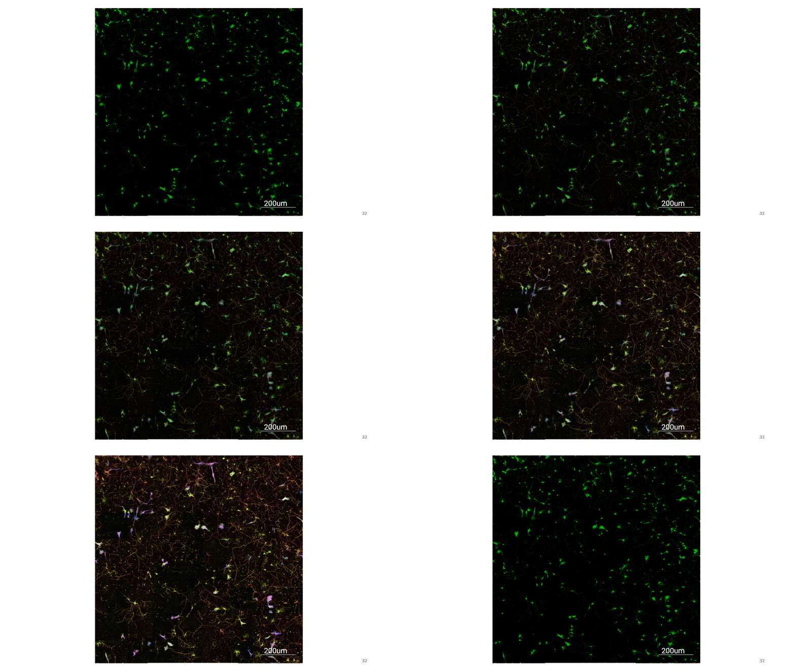
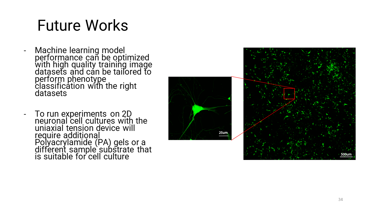
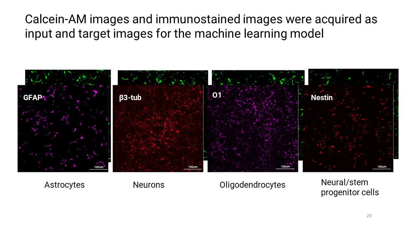
These are the images that I acquired with the microscope for the deep learning model where each immunofluorecent image for a phenotype-specific stain has its Calcein-AM image counterpart.

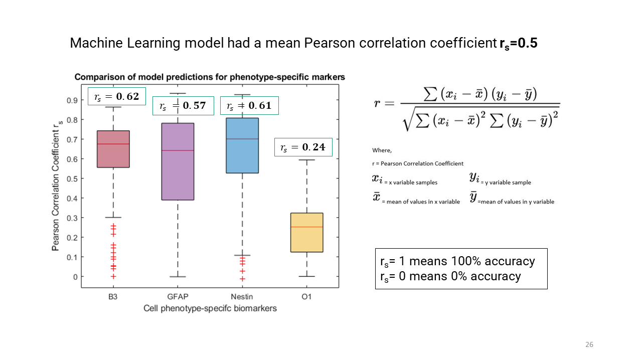
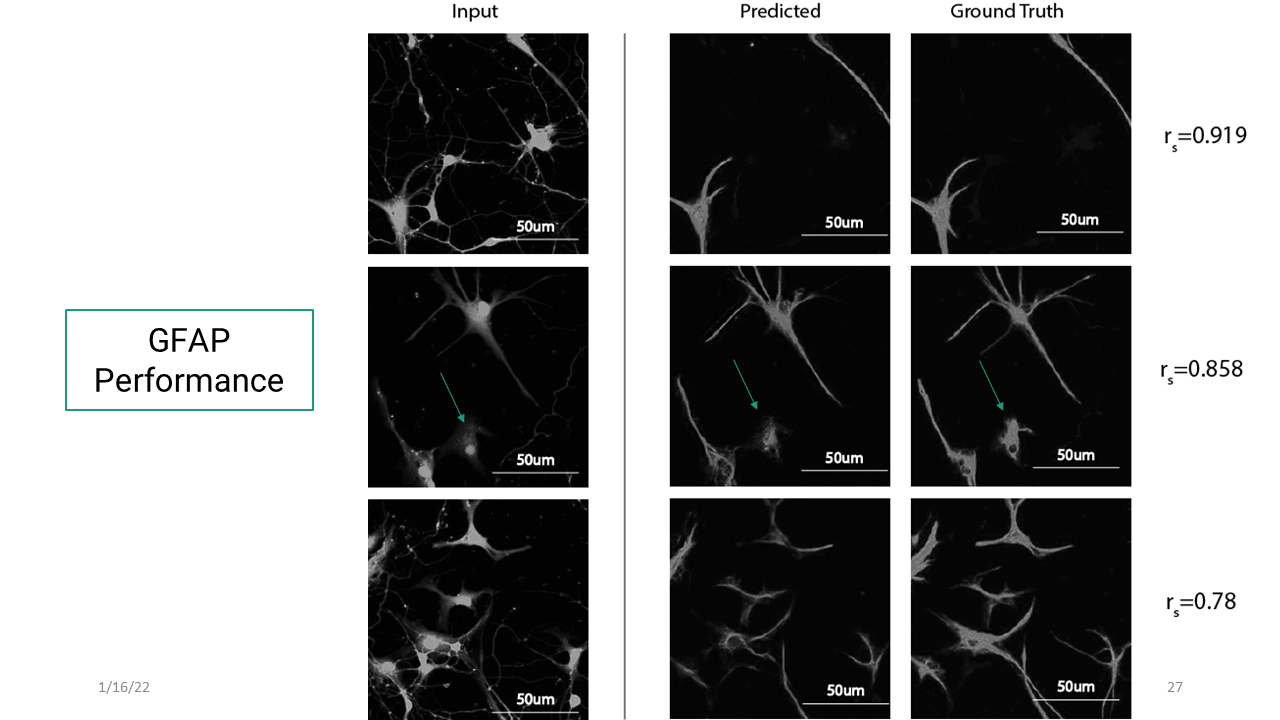
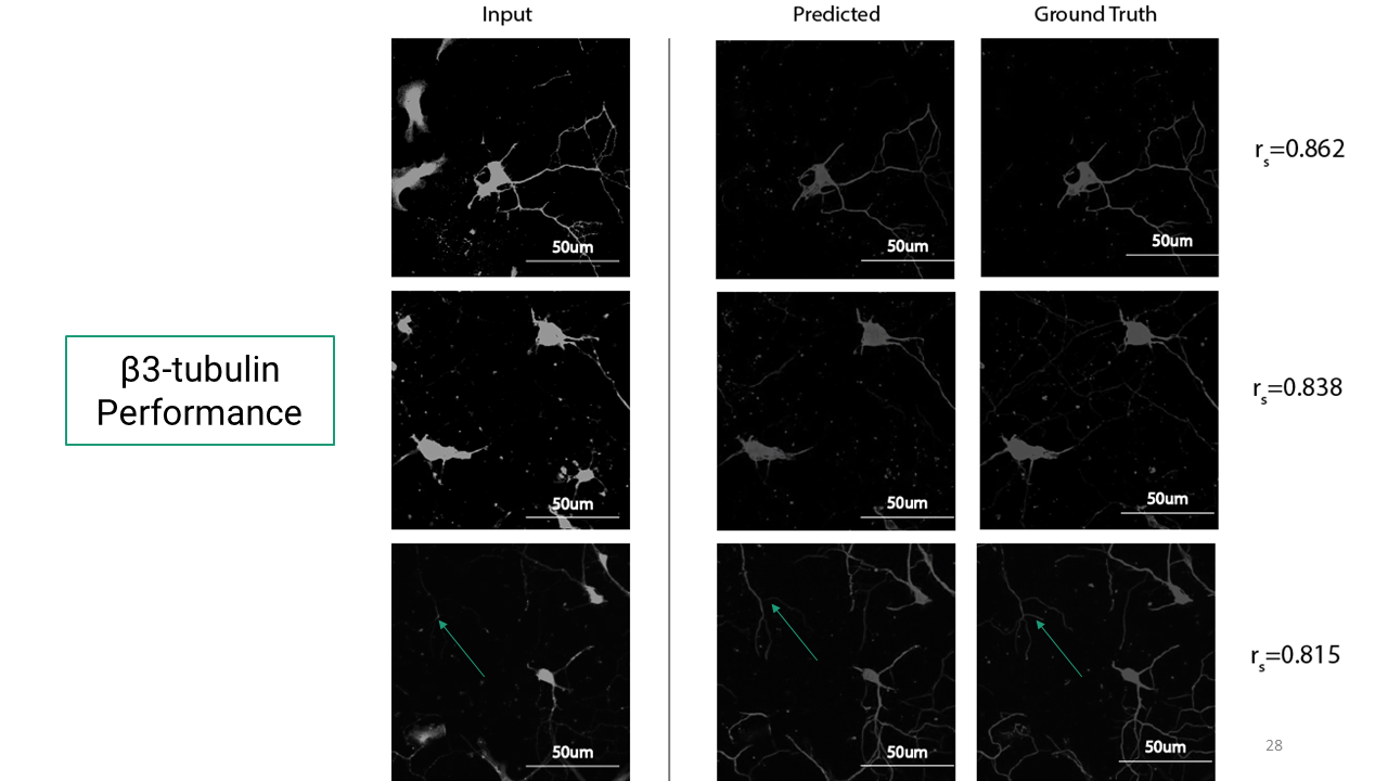
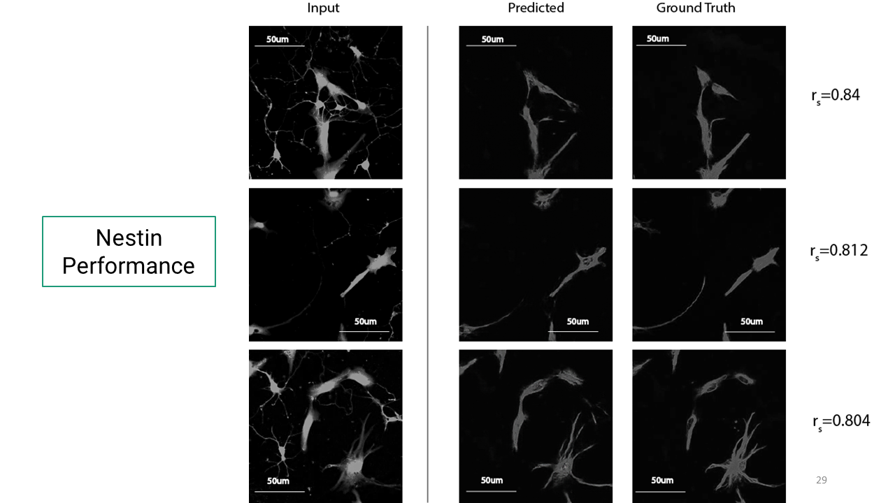
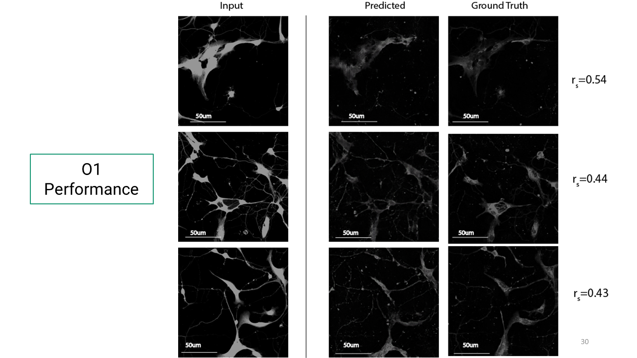
To quantify how well the trained models predicted target images, Pearson correlation coefficient was used as defined below. Rs=1 is 100% accuracy and rs=0 0% accuracy.

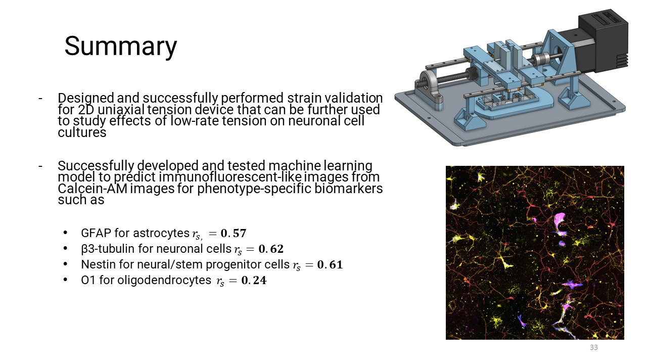
Here are the results from the deep learning model for phenotype-specific markers.

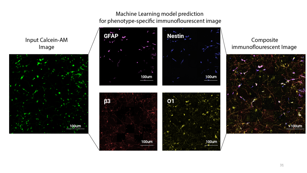
Now that I had these trained models for these markers, I wanted to see if I could get a composite immunofluorescent image as an output. So I used this Calcein-AM image as an input and this was the resulting image. (Just to note, that the colored images you see here were color adjusted in the postprocessing, after it has gone through the deep learning network).

This is a cool video to showcase how the deep learning model can predict the immunofluorescence of phenotype-specific markers: